Let’s start with the truth they don’t always tell you: Differential Equations are the hidden grammar of the universe. They’re not just an abstract math course—they’re the language in which physics whispers, biology breathes, and engineering calculates its margins of safety. This past paper isn’t a test of memorization; it’s a test of translation. Can you take a real-world phenomenon—a cooling cup of coffee, a swinging pendulum, the spread of a rumor—and decode its behavior into mathematics, then solve for its future?
Forget the idea that this is just “harder calculus.” This is where calculus graduates from finding slopes to predicting outcomes.
What This Paper Actually Solves: The Art of Modeling Change
1. The Foundation: Classifying the Universe of Equations
The first step is always diagnosis. You’ll be thrown an equation and must immediately recognize its type, because the strategy for solving it depends entirely on this.
- ODE vs. PDE: Is this a function of one variable (Ordinary) or several (Partial)? PDEs (like the heat equation) are the province of advanced physics, but ODEs are your core toolkit.
- Order & Linearity: Is it a first-order equation describing a rate of change, or a second-order equation dealing with acceleration and forces? Is it linear (amenable to superposition of solutions) or nonlinear (often requiring clever tricks or numerical methods)?
- Key First-Order Types: You must spot them instantly:
- Separable: The classic “get all the *y*’s with dy, all the *x*’s with dx.”
- Exact & Integrating Factors: For when the equation is almost a perfect derivative.
- Linear First-Order: The workhorse format dy/dx + P(x)y = Q(x), solved with a specific integrating factor formula.
2. The Core Toolkit: Solution Methods as Specialized Instruments
Each type of equation has its own “key.” The paper tests your fluency in selecting and using it.
- Second-Order Linear Homogeneous ODEs with Constant Coefficients: Arguably the most important block. You’ll solve the characteristic equation *ar² + br + c = 0* and interpret its roots:
- Real & distinct roots: Exponential growth/decay solutions.
- Complex roots: Oscillatory solutions (sines and cosines)—the heart of spring-mass systems and electrical circuits.
- Repeated real roots: Requiring the xe^(rx) trick.
- Non-Homogeneous Equations: The “Undetermined Coefficients” and “Variation of Parameters” methods. This is where you find the particular solution that accounts for an external forcing term (like a motor driving a spring).
- Laplace Transforms: The powerful “algebraic” weapon. You’ll transform a nasty differential equation with initial conditions into a simple algebraic equation, solve it, and then transform back. It’s like having a universal remote for solving linear ODEs, especially with discontinuous forcing functions.
3. The Application: From Abstract Math to Tangible Reality
This is where the subject earns its keep. The paper will present word problems—modeling scenarios.
- Growth & Decay: Population models (Malthusian, Logistic), radioactive decay, Newton’s Law of Cooling.
- Mixing Problems: Salt in a tank, pollutants in a lake.
- Mechanical Vibrations: Spring-mass-damper systems. You’ll derive the equation m*x” + c*x’ + k*x = F(t) and interpret solutions as under-damped, over-damped, or critically damped.
- Electrical Circuits: LRC circuits are directly analogous to mechanical systems, governed by the same second-order ODEs.
4. The Numerical Reality: When Algebra Fails
Not all equations have nice, closed-form solutions. The paper may introduce the concept of numerical methods (Euler’s method, Runge-Kutta basics) to approximate solutions—acknowledging that in the real world, the computer is your primary solver.
The Paper’s True Challenge: Strategic Problem-Solving
The difficulty isn’t the calculus; it’s the multistep strategic thinking. A single problem might require:
- Modeling: Translating a paragraph into an equation.
- Classification: Identifying the type of ODE.
- Solution: Executing the correct method flawlessly.
- Application of Initial/Boundary Conditions: Finding the specific, not just general, solution.
- Interpretation: Describing the physical behavior of the solution (e.g., “The population stabilizes at 10,000.”).
How to Master This Past Paper:
- Become a Classification Expert. Your first 10 seconds on any problem should be spent labeling it: “Ah, this is a second-order linear homogeneous with constant coefficients and complex roots.” This dictates your entire plan.
- Practice the “Word Problem to Equation” Translation. This is a separate skill from solving. Read problems slowly, identify the rate of change (dSomething/dt), and the law governing it (rate is proportional to…).
- Memorize the Solution Forms, Not Just Steps. Know that the solution to *y” + ω²y = 0* is A cos(ωt) + B sin(ωt). Pattern recognition saves precious time.
- Set Up Your Solutions Neatly. A misplaced negative sign in the characteristic equation will cascade. Line-by-line, disciplined work is non-negotiable.
- Connect to the Physical World. When you solve a spring equation, don’t just write the answer. Know that a negative exponent means the oscillations die out (damping). This understanding helps you spot if your answer is physically plausible.
This past paper is your proof of predictive power. It demonstrates you can move beyond describing how things change to mathematically dictating what they will become. Solving it means you’re not just a mathematician—you’re a modeler of reality.
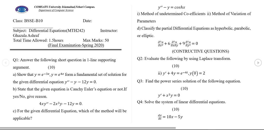
Differential equations Mid Term Examination 2021
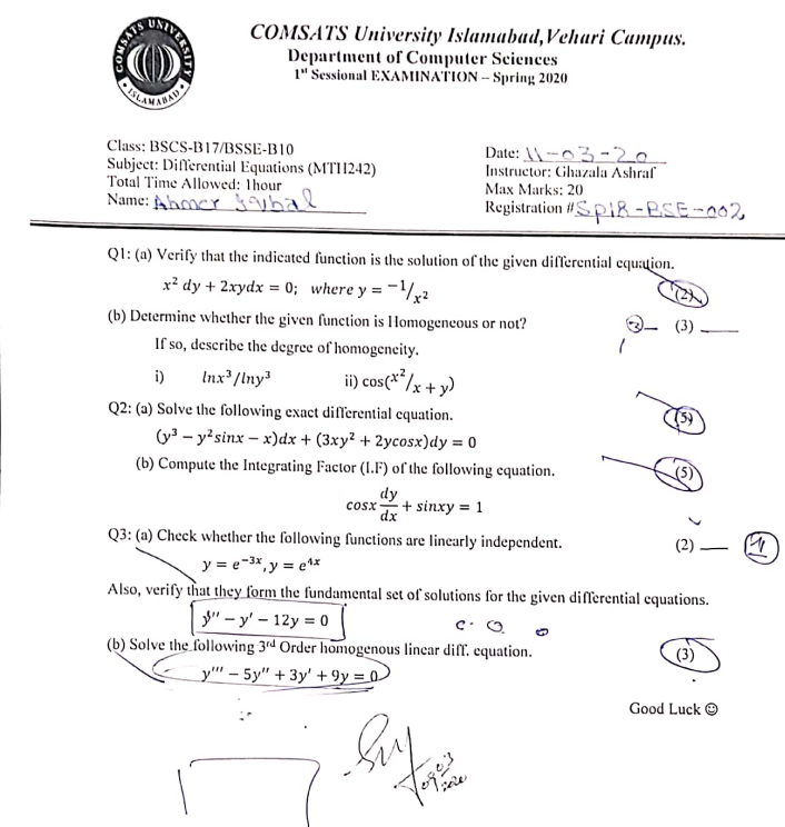
Sessional 1 2020
Sessional 2 2020