Paper Of Numerical Computing Department Of Computer Science and Software Engineering

Let’s get this straight: Numerical Computing is where the perfect, pristine world of mathematics collides with the gritty, finite reality of computers. It’s not about getting the answer; it’s about getting a good enough answer, knowing how good it is, and not setting your computer on fire in the process. This past paper is your stress test for doing real, useful math with machines that can’t even represent the number 0.1 perfectly.

Forget symbolic algebra and neat closed-form solutions. This is the toolbox for simulating galaxies, predicting weather, training AI, and valuing financial derivatives—all problems where “just solve the equation” is a fantasy.

What This Paper Actually Calculates: Your Pragmatic Math Intelligence

1. The Foundation: Sources of Error (The Real Enemy)
The first questions attack the core truth: All numerical answers are wrong. Some are useful. You must diagnose and quantify the error:

• Rounding Error: Inevitable from finite-precision arithmetic (floating-point). You’ll explain why (0.1 + 0.2) != 0.3 and analyze catastrophic cancellation.
• Truncation/Discretization Error: From approximating infinite processes (infinite series, infinitesimal steps) with finite ones. The error of cutting off a Taylor series or approximating a derivative.
• Stability & Condition Number: Does the algorithm magnify small errors? Is the problem itself sensitive to input perturbations? You’ll calculate condition numbers and identify ill-conditioned systems.

2. The Core Toolkit: Solving Problems Computers Can’t “Solve”
The paper tests your mastery of replacing unsolvable problems with solvable approximations.

A. Equations & Optimization:

• Root-Finding: Bisection (slow, bulletproof), Newton-Raphson (fast, needs a good guess and the derivative). You’ll perform iterations by hand and analyze convergence.
• Systems of Linear Equations: Gaussian Elimination with Partial Pivoting (to avoid instability), understanding LU Decomposition. You’ll solve a small system and discuss computational complexity (O(n³)).
• Eigenvalues & Eigenvectors: Power method for dominant eigenvectors. Understanding their use in stability analysis, PageRank algorithms, and principal component analysis.

B. Approximation & Data:

• Interpolation: Constructing polynomials (Lagrange, Newton’s Divided Difference) that pass exactly through data points. Knowing the perils of high-degree polynomials (Runge’s phenomenon).
• Curve Fitting / Regression: Least Squares approximation. You’ll set up and solve the normal equations to fit a line or polynomial to noisy data.
• Numerical Differentiation & Integration:
  • Differentiation: Finite-difference formulas (forward, backward, central) and their error terms (O(h) vs. O(h²)).
  • Integration: Trapezoidal Rule, Simpson’s Rule (higher accuracy). You’ll apply them and calculate error bounds.

C. Differential Equations (The Workhorse of Science):

• Ordinary Differential Equations (ODEs): Euler’s method (simple, low accuracy), Runge-Kutta methods (especially 4th order – the workhorse). You’ll perform step-by-step iterations to approximate a solution.
• Partial Differential Equations (PDEs): Introduction to discretizing Laplace’s or the Heat Equation using Finite Difference Methods, leading to a large system of linear equations.

3. The Implementation Mindset: Algorithms Over Formulas
You are tested on turning mathematical ideas into concrete, step-by-step algorithms. You’ll write pseudocode for methods like Newton-Raphson or Gaussian elimination, paying attention to loops, stopping criteria (|xₙ₊₁ - xₙ| < tolerance), and avoiding division by zero.

4. Analysis: The “Why” Behind the Method
For every technique, you must know:

• Cost: How many floating-point operations (flops)? Is it O(n²) or O(n³)?
• Accuracy: What is the order of convergence/error? (O(h²) means halving the step h quarters the error).
• Trade-offs: Speed vs. stability, memory vs. accuracy.

The Paper’s Real Challenge: Multi-Step Problem Solving
The hardest questions are synthesis problems. For example:
*”Given this differential equation modeling a pendulum, derive the finite difference approximation. Using a step size of h=0.1 and the 4th-order Runge-Kutta method, perform two iterations. Then, discuss how you would verify the stability of your numerical solution.”*
This combines modeling, algorithm application, and critical analysis.

How to Conquer This Past Paper:

1. Embrace Approximations. Let go of the desire for exactness. Your goal is a controllable error bound.
2. Perform Hand Iterations Fluently. Practice carrying out 3-4 steps of a method (Newton, Euler, Gaussian Elimination) neatly and accurately. Exam success depends on this manual execution.
3. Master Error Terminology. Be precise: “The truncation error is O(h²), but due to rounding error, there is an optimal h below which the total error increases.”
4. Connect Methods to Motives. Don’t just memorize steps. Know when to use what: Need a robust root? Use Bisection. Need a fast root with a good guess? Use Newton. Fitting experimental data? Use Least Squares.
5. Write Clean, Indexed Pseudocode. Use k for iteration counters, x_k for iterates. Clearly state inputs, outputs, and stopping conditions.

This past paper is your certification in practical computation. It proves you have the humility to accept error, the skill to minimize it, and the wisdom to measure it. Passing it means you are equipped to turn the unsolvable problems of science and engineering into actionable, computational results.

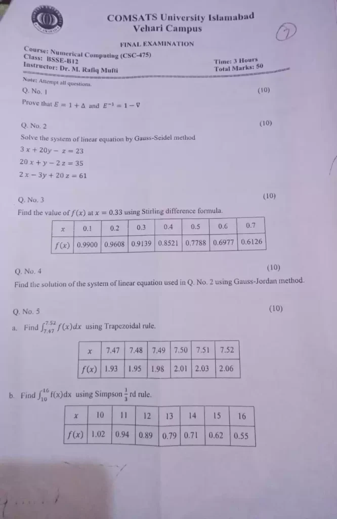
Numerical Computing Fall 21 past paper

Numerical computing final paper

1. Solve the following system using Jacobi method (with 4 digu roues arithmetic, at least). Assume the error tolerance as 0.0001.

15x₁-2X2-6Xj+0x₁ -2x)+12×2-4X3-X4=300

0 -6×1-4×2+19×3-9×4 =0

0x1-X2-9X3+21x₁=0

(Marks 10)

2. Obtain the first and second derivative at x-7 using Stirling formula. Where

Xp= 12

X

5

6

7

8

9

10

f(x)

196

394

686

1090

1624

2306

(Marks-10)

x

3. Use the table in Question no. 2 of values by Newton forward differentiation formula. To compute f (0.25), (0.50), (0.75).

2125 (Marks= 15)

4. Use Question no. lequations, to find X1, X2, X3, and x, values using Gauss

Jordan Elimination Method.

(Marks 10)

5. Compute ff(x) dx based on Trapezoidal rule. 0.6

X

0

0.1

0.2

0.3

0.4

0.5

0.6

f(x)

0

0.0998

0.1987 0.2955 0.38994

0.4794

0.5646

(Marks-05)

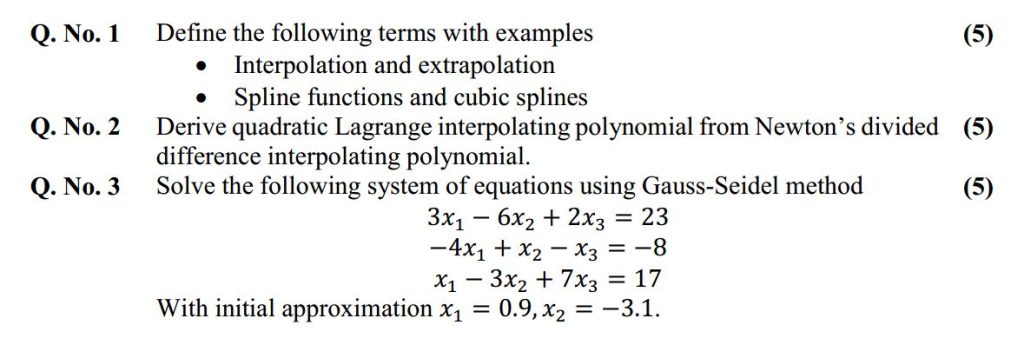
Numerical Computing  Mid term paper

Numerical Computing Sessional 1 question paper

Numerical Computing Sessional 2 question paper

1. Filling the blanks (Score: 2 5=10)

(1)     Let ξ=g(ξ)∈[a, b] be a fixed point of the real-valued and continuous function g(x). If g(x) has a continuous derivative in some neighborhood of ξ with ________.

Then the sequence (x_k) defined by x_k+1=g(x_k) converges to ξ as k→∞, provided that x₀ is sufficiently close to ξ.

(2)     Assume that .Let be distinct real numbers and suppose that are real numbers. Then, there exists a unique Lagrange polynomial such that ____________.

(3)     Suppose that a real-valued function g(x) has a fixed point ξ in [a, b]. Then, the corresponding expression can be written as________.

(4)     Given that 4x²-a=0, where a is positive real number. Then, the iteration for solving this equation by the secant method can be expressed as ____________with x₀ and x₁ being the starting values.

(5)     During the process of finding the single solution to the equation f(x) =0 in [a₀, b₀] with f(a₀)f(b₀)<0, the first step is to consider the midpoint . If (the given tolerance), then we need to choose the new interval:[a₁, b₁]=[a₀, c₀] in the case of _____;or [a₁, b₁]=[c₀, b₀] in the case of _____.

1. Find solution using Bessel’s formula Score= 10
2. Find Solution using Newton’s Backward Difference formula    Score=10

x = 4.75

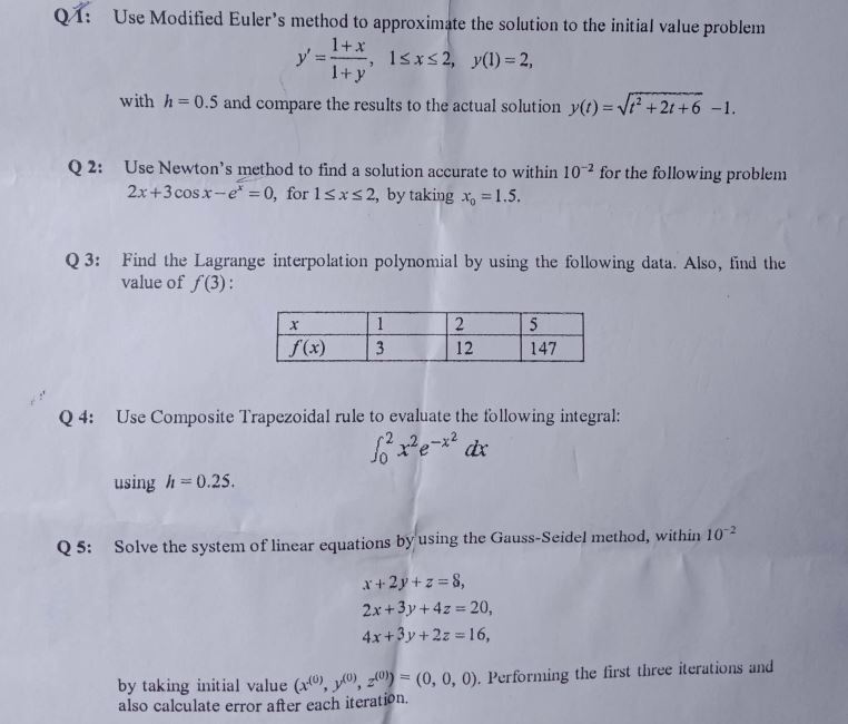
Numerical Computing Final question paper

1. MCQ’s (Marks=10)
   204. How much significant digits in this number 204.020050?
        1. 5
        2. 7

• 9

1. 11
2. In which of the following method, we approximate the curve of solution by the tangent in each interval.
   1. Hermite’s method
   2. Euler’s method

• Newton’s method

1. Lagrange’s method

1. When   do   we   apply   Lagrange’s   interpolation?
   1. Evenly spaced
   2. Unevenly spaced

• Both

1. None of above
2. When   Newton’s   backward formula is used?
   1. To interpolate values
   2. To calculate difference

• To find approximate error

1. None of above

1. What are the errors in Trapezoidal rule of numerical integration?
   1. E<Y
   2. E>Y

• E=Y

1. None of above

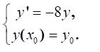
2. Consider the initial value problem; give the condition of the absolute stability for the Euler method. (Marks= 10)

2. Suppose that the function values of f(x) are given in the following table.

(Marks= 10)
Find the approximate function value at the point  by the Lagrange’s interpolation polynomial of degree 2.

4. Use the predictor-corrector method to get the approximate solution of the following initial value problem (Marks= 10)

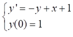            with h = 0.1, 0 < x < 0.5.

5. Consider the function f(x) = cos x−x=0. Approximate a root of f(x) via Newton’s Method. (Marks= 10)

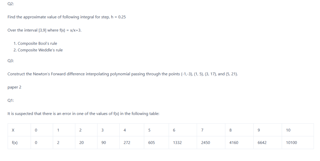
Numerical Computing Final Paper 2022